Scope
Bilevel optimization problems are commonly found in many practical problems appearing in transportation (network design, optimal pricing), economics (Stackelberg games, principal-agent problem, taxation, policy decisions), management (network facility location, coordination of multi-divisional firms), engineering (optimal design, optimal chemical equilibria) etc. Below we have highlighted some of the practical bilevel problems that have been studied in the literature.
Toll Setting Problem

This problem involves finding the optimal tolls for a network of roads operated by an authority, which may be the government or a company. In this problem the authority is an upper level decision maker, and the network users (drivers) are the lower level decision maker. The authority is aware that for any given toll the network users try to minimize their own travel costs. Therefore, the authority desires to optimize its revenues earned by tolls by taking the network users' problem into account (Brotcorne et al. 2001).
Consider that the upper level variable is given by , where represents the toll introduced by the authority on a network. The lower level variable is given by , where is the extent to which the road network provided by the authority is used, and represents the extent to which an alternative route is used. There is a fixed cost which the users incur while using , and a fixed cost which the users incur while using . The authority wants to maximize its revenues and the users want to minimize their costs. The bilevel formulation for such a toll setting problem can be stated as follows:
In the above formulation, , and are constants in the lower level constraints. The toll users need to satisfy these constraints while optimizing their own problem.
Stackelberg Duopoly

Leader-follower (Stackelberg 1952) models are a classic real-life example of bilevel programming. In such problems, the upper level contains the leader’s problem and the lower level contains the follower’s problem. It is a strategic game, where the leader makes the first move and has all relevant information about the possible actions the follower might take in response to his own actions. On the other hand, the follower usually observes and reacts optimally to the actions of the leader. The leader solves a Stackelberg competition model in order to determine the optimal actions which he should take.
Below, we consider a simple Stackelberg competition model (Sinha et al. 2013; Frantsev et al. 2012) in a single time period, where the leader and follower firms compete solely by choosing their production levels. Formally, this model can be presented as follows:
where is the quantity demanded, is the price of the goods sold, and is the cost of production of the respective firm. The variables in this model are the production levels of each firm , and demand . The leader sets its production level first, and then the follower chooses its production level based on the leader's decision. This simple model assumes homogeneity of the products manufactured by the firms. Additionally, the upper level constraint ensures that all demand is satisfied. By assuming that the firms produce and sell homogeneous goods, a single linear price function for both firms can be specified as an inverse demand function of the form
where are constants. Additionally, since costs often tend to increase with the amount of production, one assumes convex quadratic cost functions for both firms to be of the form
where denote the fixed costs of the respective firm, and and are positive constants.
Optimal Chemical Equilibria

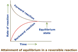
In a chemical reaction, the chemists have to decide upon the quantities of reactants to be used in order to optimally create one or more products. The products are produced as a result of a reaction when the reactants and products are in equilibrium. The equilibrium is established when the entropy functional is minimized subject to the mass conservation constraints. The equilibrium established depends on variables such as pressure, temperature, quantity of reactants etc.
It is possible to formulate an optimal chemical equilibria problem as a bilevel programming problem (Dempe 2002). The lower level problem involves optimizing the entropy functional to ensure that an equilibria is established. The upper level problem involves optimization of an objective such as maximizing the quantity of a particular product. Variables such as pressure, temperature, quantity of reactants etc. are the upper level variables in the bilevel program. The quantities of substances in the reactor when the equilibrium is established are the optimal lower level variables.
Environmental Economics

Bilevel programming problems commonly appear in environmental economics. For instance, consider a regulating authority, which wants a mining company to operate in a manner such that the environmental damage is minimal (Sinha et al. 2013). The regulating authority cannot completely stop the mining activity as it earns revenues from the mining company in the form of taxes. Under such a situation, this problem can be formulated as a bilevel problem with multiple objectives at the upper level.
The regulating authority has primarily two objectives: the first objective is to maximize the revenues generated by the mining project, which may include the additional jobs, taxes, etc; and the second objective is to minimize the harm caused to the environment as a result of mining. Obviously, there is a trade-off between the two objectives, and the authority as a decision maker needs to choose one of the preferred trade-off solutions. The authority is aware that the mining company has a sole objective of maximizing its profit under the given constraints. In this scenario, the authority would like to decide upon a tax structure such that it is able to maximize its own revenues in addition to being able to restrain the mining company from causing extensive damage to the environment. There is a hierarchy in the problem, which arises from the manner in which the two entities operate. The regulating authority has higher control of the situation and decides the terms and conditions for the mining company to operate in. Therefore, in this framework, we observe that the regulating authority acts as a leader, and the mining company acts as a follower.
As a leader, it is possible for the authority to optimally regulate the problem in its favour, provided that it has a complete knowledge of the follower's strategies. If the government decides to tax the mining company based on each unit of the product it produces, then for any given tax structure, the mining company will solve its own optimization problem to maximize its profit. However, if the authority already takes the mining company's optimization task into account, then it would be possible for them to generate their own optimal strategies. The overall problem appears as a bilevel optimization task, where for each tax structure, the government observes how the company acts and then chooses that particular tax structure which suits it the most, taking the actions of the mining company into account. A basic bilevel model for this can be formulated as follows:
where, at the upper level, the first objective is the tax revenue, such that is the tax per unit of metal extracted, and is the amount of metal extracted from the ore by the latter. The second objective denotes the environmental damage caused by the mine that the government ultimately wants to minimize, such that is the pollution coefficient (constant) signifying the negative impact of extraction on the environment. The lower level objective gives the profit of the mine, where (price function times amount of metal extracted) is the revenue function, and is the extraction cost function followed by the additional tax ( ) levied on the mine.
Structural Optimization

Structural optimization problems are inherently a bilevel optimization problem in nature (Hlaváček et al. 1988; Bendsøe 1995; Christiansen et al. 2001). Such problems commonly involve minimizing the weight or cost of a structure at the upper level by searching for the most suitable design variables. The decision variables at upper level in structural optimization problems usually are shape of the structure, choice of materials, amount of material etc. The constraints at the upper level involve bounds on displacements, stresses and contact forces. The displacements, stresses and contact forces are referred as state variables, and their values are found by minimizing the potential energy of the system. The equilibrium satisfaction or the potential energy minimization problem appears as a lower level optimization problem with the state variables appearing as lower level decision variables.
Structural optimization problems have been traditionally modeled as single-objective optimization problems by replacing the lower level optimization task with its KKT conditions. They are commonly referred as mathematical programming problems with equilibrium constraints (MPEC) and a number of approximate procedures have been developed to handle such problems. However, most of the available solution procedures are limited to handling relatively simple versions of the problem.